
 E-mail Alert
 RSS
RSS
-
摘要
利用深度学习进行超分辨重建已经获得了极大的成功,但是目前绝大多数网络结构依然存在训练以及重建速度较慢,一个模型仅能重建一个尺度以及重建图像过于平滑等问题。针对这些问题,本文设计了一种级联的网络结构(DCN)来逐级对图像进行重建。使用L2和感知损失函数共同优化网络,在每一级的共同作用下得到了最终高质量的重建图像。此外,本文的方法可以同时重建多个尺度,比如4×的模型可以重建1.5×,2×,2.5×,3×,3.5×,4×。在几个常用数据集上的实验表明,该方法在准确性和视觉效果均优于现有的方法。
Abstract
Convolutional neural networks have recently been shown to have the highest accuracy for single image super-resolution (SISR) reconstruction. Most of the network structures suffer from low training and reconstruction speed, and still have the problem that one model can only be rebuilt for a single scale. For these problems, a deep cascaded network (DCN) is designed to reconstruct the image step by step. L2 and the perception loss function are used to optimize the network together, and then a high quality reconstructed image will be obtained under the joint action of each cascade. In addition, our network can get reconstructions of different scales, such as 1.5×, 2×, 2.5×, 3×, 3.5× and 4×. Extensive experiments on several of the largest benchmark datasets demonstrate that the proposed approach performs better than existing methods in terms of accuracy and visual improvement.
-
Key words:
- deep learning /
- super-resolution /
- step by step /
- multi scale /
- perception loss function
-
Overview
Overview: Recovering high resolution (HR) image from its low resolution (LR) image is an important issue in the field of digital image processing and other vision tasks. Recently, Dong et al. found that a convolutional neural network (CNN) can be used to learn end-to-end mapping from LR to HR. The network is expanded into many different forms, using sub-pixel convolutional network, very deep convolutional network, and recursive residual network. Although these models have achieved the desired results, the issues still exist some problems as described as following. First, most methods use up-sampling operators, such as bi-cubic interpolation, to upscale the input image to the bigger size. This pre-processing adds considerable unnecessary computations and often results in visible reconstruction artifacts. To solve this problem, there are several algorithms such as ESPCN using sub-pixels and FSRCNN with transposed convolution. However, the network structures of these methods are extremely too simple to lean complex and detailed mappings. Second, most existing methods use only L2 to optimize the network, which will result in an excessively smooth image less suitable for human vision. Third, those methods cannot reconstruct more than one scale, which means a model is only for one scale, and this will increase the extra-works of training for the other scales, especially for large-scale training.
To address these defects, we propose a deep cascaded network (DCN). DCN is a cascade structure, and it takes an LR image as input and predicts a residual image in each scale. The predicted residual for each scale is used to efficiently reconstruct the HR image through up-sampling and adding operations. We train the DCN with L2 and perceptual loss function to obtain a robust image.
Our approach differs from existing CNN-based methods in the following aspects:
1) Multiple scales with cascade layers. Our network has a cascade structure and generates multiple intermediate SR predictions in feed-forward process. This progressive reconstruction can get more accurate results. Our 4× model can obtain 1.5×, 2×, 2.5×, 3×, 3.5× reconstructed images.
2) Optimize network with L2 and perceptual loss function. Using L2 can get more accurate pixel-level reconstruction and using perceptual loss function may be closer to human vision.
3) Features extraction on LR image. Our method does not require traditional interpolation methods to up-sample images as a pre-processing, thus greatly reducing the computational complexity.
Extensive experiments on several large benchmark datasets show that the proposed approach performs better than existing methods in terms of accuracy and visual improvement.
-
1. 引言
从低分辨率图像中恢复高分辨率图像是数字图像处理领域的一个重要课题。近年来,基于实例的超分辨重建方法通过从大量图像数据中学习低分辨率(low resolution, LR)到高分辨率(high resolution, HR)的映射,表现出最先进的性能,比如随机森林[1],邻域嵌入[2-3],稀疏编码[4-7]。最近,Dong等人首先证明卷积神经网络(convolutional neural network, CNN)可以端到端地学习一系列滤波核参数来进行超分辨重建,并设计了一种超分辨重建网络结构(super-resolution convolutional neural network, SRCNN)[8-9]。这种网络结构被扩展为很多形式:比如使用子像素神经网络(efficient sub-pixel convolutional neural network, ESPCN)[10],使用超深结构的网络(very deep convolutional network for super-resolution, VDSR)[11]和DRRN(deep recursive residual network)[12],使用循环结构的神经网络(depth recursive convolution network, DRCN)[13]和DRRN[12]等。
SRCNN仅包含3层,分别是特征提取层,非线性映射层,重构层。卷积核大小分别是9×9,1×1和5×5。由于网络深度很浅,提取的特征有限。VDSR将网络增加到了20层并使用了残差结构来提高网络训练速度,同时通过增加多个尺度数据来训练网络使得网络能够重建多个尺度。DRRN在此基础上将网络深度提高到了52层并使用了循环结构来减少训练参数的大小。这些网络都取得了很好的效果,但是由于网络的输入是使用传统算法插值后的图像,这就增加了很多计算开销。为了解决这个问题,ESPCN网络使用子像素卷积网络,该网络直接输入低分辨率的图像,在网络最后使用子像素层对图像进行放大。FSRCNN[14]同样使用低分辨率图像作为网络输入,在网络最后一层使用一个反卷积层对图像进行上采样,这样极大地降低了计算量,使得实时重建成为可能。
尽管这些网络结构在不同方面都取得了很大的成功,但是仍然存在几个问题:
1) 大多网络使用L2作为损失函数来优化网络,会导致重建的图像过于平滑,不符合人类视觉;
2) 大多网络训练一个模型仅能重建一个尺度,增加了网络训练的复杂度;
3) 目前的网络重建一个大的尺度都是直接学习来重建最终的结果,增加了训练收敛的速度。
针对这些问题,本文设计了一种级联结构的网络(deep cascaded network, DCN),网络使用低分辨率图像(LR)作为输入,在每一个尺度级别分别重建一个上采样图像与真实图像之间的残差。且每一级都使用L2和感知损失函数[15]来共同优化网络。在每一级的共同优化下网络训练速度有了明显的提升。
经过大量实验验证,本文的方法不管在重建图像量化指标还是视觉效果较现有的网络都有很大的提高,对于图像后期处理具有一定的实用价值。
2. DCN算法描述
定义IHR是原始高分辨率图像,ILR是对应的下采样的低分辨率图像,在超分辨重建的任务中我们首先需要建立IHR和ILR对应的关系,在单帧超分辨重建中忽略掉图像的几何扭曲,因此可以将图像获取过程中的退化现象模拟为ILR经过光学模糊、下采样和噪声干扰等一系列过程,用数学表达式表示为
ILR=D∗B∗IHR+N, (1) 式中:D为下采样因子,B为模糊因子,N为噪声。从式(1)可以得到:
IHR=ILRD∗B−ND∗B, (2) 从式(2)可以看出,超分辨重建的目的就是去除ILR中的噪声N和模糊B并将其上采样1/D来得到IHR图像,Dong等人提出的SRCNN[8]中证明可以通过训练多个卷积核对图像进行滤波来去除模糊和噪声。本文中也通过训练多个卷积核来完成去噪和去模糊的过程。FSRCNN[14]中提出并验证了使用一个或者若干个反卷积核可以对图像进行一定的上采样且达到了较好的效果。本文在进行1/D上采样时也采用了一个反卷积核。在采用多个卷积和一个反卷积的基础上,本文提出了一种全新的级联网络,在下一节中将对网络进行详细说明。
2.1 DCN网络模型
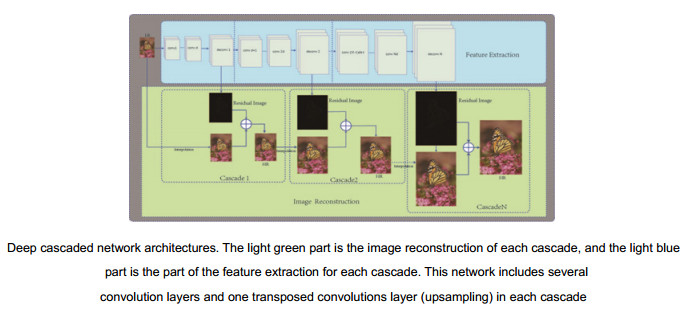
本文提出了一种多级重建网络(DCN),结构如图 1所示,该网络训练一个逐级放大的网络来逐步重建最终图像,这样可以逐级有效地消除插值带来的噪声和模糊。DCN有别于其他使用深度学习进行超分辨重建的方法,逐级的估计残差图像,例如,在4×超分辨重建任务中,网络分为6级重建,分别重建为1.5×,2×,2.5×,3×,3.5×,4×。在每一级都包含两个部分:特征的提取和图像的重建。
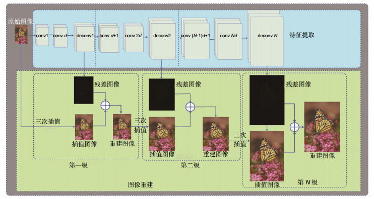 图 1. 本文级联的网络结构。浅蓝色部分为特征提取部分,浅绿色为图像重建,网络每一级都包含d个卷积层conv和一个用于上采样的反卷积层deconvFigure 1. Deep cascaded network architectures. The light green part is the image reconstruction of each cascade, while the light blue part is the part of the feature extraction and for each cascade. This network includes several convolution layers and one transposed convolutions layer (upsampling) in each cascade
1) 特征提取:
在一个特定的尺度S下,将S分为N个级别{S1,S2,...,SN},特征提取在每一级包含d个卷积层(图 1中的conv)和1个可以将特征上采样的反卷积层(图 1中的deconv),每级的输出包含两个部分,一部分用于重建这一级尺度的目标图像与传统插值图像之间的残差,另一部分直接输入到下一级重建网络中。与以往网络不同的是,每一级别中,仅有一个反卷积层将特征进行上采样,其他d个卷积层都只在低分辨率上提取特征,这样大大减少了计算复杂度。此外,每一个低级别的上采样都和高级别的上采样共享特征,共同优化网络,因此可以学习到更加复杂的非线性映射。
2) 图像重建:
在第Si级中,第Si−1层图像经过反卷积得到一个上采样到第Si级尺度,利用传统插值方法将Si−1重建的图像上采样到Si级对应的大小,并利用L2损失函数和感知损失函数联合所有其他层对网络参数进行优化。上采样的图像与预测的残差图像相加得到高分辨率的输出图像。然后将Si级的特征输出送入Si+1的图像重建级。整个网络是一个级联结构,在每一级具有类似的结构。
2.2 损失函数
在以往的基于深度学习的文章中,都使用L2作为损失函数来优化整个网络。由于L2是逐像素求差,无法从更抽象的感知层来衡量图像之间的差别。例如, 将一副图像偏移一个像素,尽管从感知上这两副图像完全一样,若使用L2来衡量的话,两幅图像就有很大的差异。人类视觉在关注图像相似度时并不是关注图像像素级的差别,而是关注更加抽象的特征,比如图像的边缘、纹理等。Johnson等人提出了一种使用特征的差别来衡量图像相似度的方法,称为感知损失函数[15]。在风格迁移和超分辨重建方面取得了较好的效果,但是由于感知损失是抽象特征的差别,忽略了像素级的差别,重建图像在像素级差别可能较大,在PSNR,SSIM等量化指标方面会较低。本文结合了L2和感知损失来优化网络。
1) L2损失函数:
定义Xsi是一个训练集中的第i张图像在第S级尺度下的对应的高分辨率图像,RSi是对应重建的残差图像,YSi是使用传统插值方法在第S级对低分辨率图像上采样的图像。则有:
L1=1nn∑i=1||(RSi+YSi−XSi)||2。 (3) 2) 感知损失函数:
定义ϕ表示一个已经训练好的卷积神经网络,通过比较重建图像经过ϕ提取的特征值与原始HR图像经过ϕ提取的特征值,使得重建图像与原始HR图像在感知层更加相似。为了和DCN的特征提取部分区分,称ϕ为感知特征取网络,本文使用ImageNet图像和VGG-19[16]训练一个感知特征提取网络。选取ImageNet数据集中的512类图像并将图像缩放到32×32,为了和DCN使用的图像Patch大小一致,随机裁剪25×25的区域进行训练,训练参数和VGG-19保持一致,ϕj表示特征提取网络第j层提取的特征,本文在提取感知特征时取VGG-19最后一层的特征,即j=19。感知损失函数定义如下:
L2=1nn∑i=1||(ϕj(RSi+YSi)−ϕj(XSi))||2。 (4) 本文使用L2和感知损失共同优化网络,损失函数定义如下:
L=L1+L2, (5) 式中:L1表示L2损失函数,L2表示感知损失函数,n表示参与训练的样本个数,本文采用随机梯度下降法来最小化损失函数。下一章节中我们比较了使用本文的损失函数和仅使用L2损失函数优化的网络模型的效果。
3. 实验结果及分析
在本节中,在多个数据集上测试本文方法的性能,首先介绍用于训练和测试的数据集;接下来介绍本文算法的实施细节;最后比较了本文方法与目前最先进的方法的效果。
3.1 训练及测试数据
按照文献[1]和[10]的方法,使用291幅图像作为训练集,其中91幅图片是来自Yang等人[17],和其他200幅来自Berkeley Segmentation Dataset[18]。测试中,使用四种广泛使用的基准数据集,Set5[2]、Set14[19]、urban100[20]以及bsd100[21],分别包含5,14,100和100张测试图像。
3.2 实施细节分析
1) 训练:
为了获得更多的训练数据,本文对291幅训练图像进行了增强处理,对图像进行镜像、反转、旋转90°、180°、270°,这样就得到了5个增强数据集。将训练图像分成25×25的像素块,每次步进21 pixels,考虑到训练时间和存储空间。设置SGD的mini-batch为64,一次循环有3600次迭代,所有卷积层的初始学习率为0.01,每30个循环学习率减少一半。实验硬件环境为CPU:7700K,GPU:1080TI,内存:32 G,深度学习架构使用Caffe[22]。
2) 卷积核参数:
在大量实验后, 对于本文的2×重建模型选择d=15,对于4×模型选择d=12。为了减少计算量,本文的网络每一级只有一个反卷积层(上采样层),我们使用不同的卷积核大小,并在不同的卷积层中选择性地填充零,以保证反卷积层后的图像大小。卷积层和反卷积层的参数如表 1所示。
表 1. 每一层的卷积核参数。其中,conv列中,d < 6?5×5:3×3表示在层数小于6时,卷积核大小是5×5,其他都是3×3;在padding列中,d < 4?0:1表示在层数小于4时,不填充0,其他填充1个0;Size表示每一级后训练图像的分辨率Table 1. Net parameters for each cascade. In the conv column, d < 6?5×5:3×3 means if d < 6, the kernel size is 5×5, otherwise is 3×3. In the padding column, d < 4?0:1 means if d < 4, we do not pad zero, otherwise pad one zero. The size in the table means the output image size for the cascadeModel Cascade Size Conv Deconv Conv stride Deconv stride Padding 2× 1.5× 38 3×3 3×3 1 2 d < 4?0:1 2× 52 3×3 3×3 1 2 d < 7?0:1 4× 1.5× 38 3×3 3×3 1 2 d < 4?0:1 2× 52 3×3 3×3 1 2 d < 7?0:1 2.5× 64 3×3 3×3 1 2 d < 11?0:1 3× 76 d < 6?5×5:3×3 3×3 1 2 d < 9?0:1 3.5× 88 d < 7?5×5:3×3 3×3 1 2 d < 11?0:1 4× 100 d < 8?5×5:3×3 3×3 1 2 0 | Show Table DownLoad:
CSV
DownLoad:
CSV
3) 级联结构:
我们训练了和最终模型有相同层数的非级联结构的网络,对于2×模型,训练了一个具有30个卷积层和1个反卷积层的非级联网络,图 2(a)中的曲线表示了级联以及非级联网络训练速度以及效果的比较,从曲线可以看出,级联网络在第15次循环后就基本已经达到了最优而非级联网络到25次循环后才达到最优,且从图上可以看出,使用级联的网络重建的峰值信噪比(peak signal to noise ratio, PSNR)要高于非级联网络。
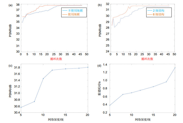 图 2. 不同网络参数对重建效果和耗时的影响(Set5数据集平均值)(a) 2×模型中使用级联和不使用级联对比;(b) 4×模型中使用两级和使用6级的对比;(c) 4×模型中网络深度对重建PSRN的影响;(d) 4×模型中网络深度对重建耗时的影响Figure 2. The effects of different network parameters on the reconstruction effect and time consuming(a) Comparison of cascade and no-cascade structure in the 2× model; (b) The comparison between 2 levels and 6 levels in the 4× model; (c) The influence of network depth on the reconstruction of PSRN in the 4× model; (d) The influence of network depth on the time consuming of the 4× model
同时本文测试了分不同级别,以4×模型为例,测试了分两级(2×,4×)以及分6级(1.5×,2×,2.5×,3×,3.5×,4×),图 2(b)可以看出分6段的训练的收敛速度以及重建效果上均优于两级模型。
4) 网络深度:
本文测试了不同的网络深度,d=5,10,12,15,18,20。从测试数据来看,网络越深,重建图像效果相对越好,同时训练以及重建耗时也就越长。图 2(c),图 2(d)中表示了不同深度对重建效果的影响。从图中可以看出在每级的深度超过12之后,PSNR增加比较少,但是耗时相对增加较多。综合效果和耗时考虑,在4×模型上选择d=12,同样经过试验得到2×模型使用d=15。
3.3 实验效果比较
分别比较了本文算法与A+[23],SRCNN[8-9],FSRCNN[14],DRCN[13],VDSR[11],DRRN[12],比较的数据集为SET5[2],SET14[19],BSDS100[20],URBAN100[21]。其中SET5,SET14以及BSD100包含一些自然场景的图像。URBAN100包含一些具有大量边缘细节的图像。我们使用两种常见的量化指标PSNR和结构相似度指数(structural similarity index measurement, SSIM)[24],表 2为2×和4×模型的比较。其中,DCN(2×/4×)表示使用2×模型还是4×模型。DCN-L2表示仅使用L2损失函数优化网络。红色的表示效果最好的,蓝色的表示效果次好的。图 3,图 4分别展示了4×模型中4×重建以及4×模型中3×重建在不同数据集上的效果。图 5中为从一个监控视频中抽取的一帧分辨率为352×288图像4×重建对比。图 6展示了本文4×模型在1.5×,2×,2.5×,3×,3.5×,4×的重建效果。
 图 3. Set5数据集中的“Baby”图片4×重建,DCN睫毛部分重建效果比其他方法稍好一些,DCN-L2在PSNR和SSIM数据指标上均低于DCN(使用L2和感知损失优化)(a)原始图像;(b) 3次插值(PSNR/SSIM:31.79/0.857);(c) SRCNN重建(PSNR/SSIM:32.98/0.878);(d) VDSR重建(PSNR/SSIM:33.42/0.889);(e) DRCN重建(PSNR/SSIM:33.51/0.889);(f) DRRN重建(PSNR/SSIM:33.53/0.889);(g) DCN-L2(仅使用L2优化网络重建)(PSNR/SSIM:33.97/0.887);(h) DCN(使用L2和感知损失共同优化重建)(PSNR/SSIM:34.11/0.893)Figure 3. "Baby" from Set5 with an upscaling factor 4, DCN can reconstruct eyelashes better, DCN- L2 is lower than DCN on both PSNR and SSIM (using L2 and perceptual loss optimization)(a) Original image; (b) Bicubic(PSNR/SSIM: 31.79/0.857); (c) SRCNN(PSNR/SSIM:32.98/0.878); (d) VDSR(PSNR/SSIM:33.42/0.889); (e) DRCN(PSNR/SSIM: 33.51/0.889); (f) DRRN(PSNR/SSIM:33.53/0.889); (g) DCN-L2(PSNR/SSIM:33.97/0.887);(h) DCN (optimizing with L2 and perceptual loss) (PSNR/SSIM:34.11/0.893)
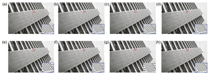 图 4. URBAN100数据集中的“img-092”图片4×模型中3×重建,DCN-L2和DCN在第十层以后的纹理处更接近真实图像,DCN(使用L2和感知损失优化)在视觉效果和PSNR/SSIM指标均高于其他方法(a)原始图像;(b) 3次插值(PSNR/SSIM:17.32/0.516);(c) SRCNN重建(PSNR/SSIM:18.48/0.619);(d) VDSR重建(PSNR/SSIM:19.68/0.702);(e) DRCN重建(PSNR/SSIM:19.54/0.606);(f) DRRN重建(PSNR/SSIM:20.09/0.721);(g) DCN-L2(仅使用L2优化网络重建)(PSNR/SSIM:20.11/0.708);(h) DCN(使用L2和感知损失共同优化重建)(PSNR/SSIM:20.14/0.728)Figure 4. "img-092" image from URBAN100 with an upscaling factor 3, DCN model is 3× reconstruction in 4× model, only DCN and DCN-L2 can correctly recover sharp lines, DCN performance is better"img-092" image from URBAN100 with an upscaling factor 3, DCN model is 3× reconstruction in 4× model, only DCN and DCN-L2 can correctly recover sharp lines, DCN performance is better. (a) Original image; (b) Bicubic (PSNR/SSIM : 17.32/0.516); (c) SRCNN(PSNR/SSIM : 18.48/0.619); (d) VDSR(PSNR/SSIM : 19.68/0.702); (e) DRCN(PSNR/SSIM:19.54/0.606); (f) DRRN(PSNR/SSIM:20.09/0.721); (g) DCN-L2(PSNR/SSIM:20.11/0.708); (h) DCN(optimizing with L2 and perceptual loss) (PSNR/SSIM:20.14/0.728)
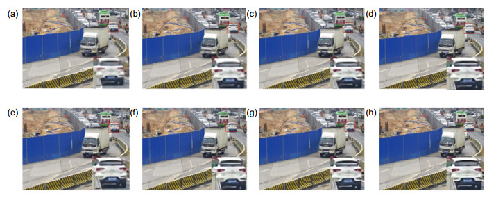 图 5. 监控视频中单帧图像4×重建,从视觉上本文的DCN在车辆后玻璃窗部分重建效果更真实(a)原始低分辨率图像; (b) 3次插值; (c) SRCNN重建; (d) VDSR重建; (e) DRCN重建; (f) DRRN重建; (g) DCN-L2(仅使用L2优化网络重建); (h) DCN(使用L2和感知损失共同优化重建)Figure 5. 4× reconstruction of single frame image in video surveillance, the visual effect of the DCN in the rear window part of the vehicle is more authentic(a) Original image; (b) Bicubic; (c) SRCNN; (d) VDSR; (e) DRCN; (f) DRRN; (g) DCN-L2; (h) DCN (optimizing with L2 and perceptual loss)
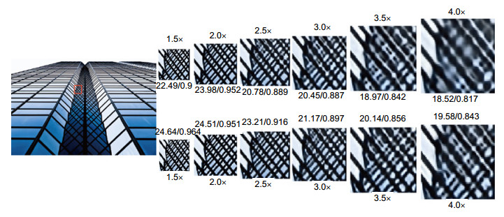 图 6. 本文4×网络在1.5×, 2×, 2.5×, 3×, 3.5×, 4×重建效果对比。第1行为使用VDSR的4×模型重建的各尺度效果,第2行为本文4×模型重建各尺度的效果Figure 6. The comparison between our model and VDSR at different scales(1.5×, 2×, 2.5×, 3×, 3.5×, 4×). The first line is the result of VDSR reconstruction. The second line is reconstructed by our model表 2. 几个数据集上的超分辨重建算法比较:分别比较2×以及4×模型的P重建PSNR/SSIM的均值Table 2. Quantitative evaluation of state-of-the-art SR algorithms: average PSNR/SSIM for scale factors 2×, 4×
Scale Method SET5 SET14 BSD100 URBAN100 PSNR/SSIM PSNR/SSIM PSNR/SSIM PSNR/SSIM 2× Bicubic 33.65/0.930 30.34/0.870 29.56/0.844 26.88/0.841 A+[16] 36.54/0.964 32.40/0.906 31.22/0.887 29.23/0.894 SRCNN[8] 36.65/0.954 32.29/0.903 31.36/0.888 29.52/0.895 FSRCNN[17] 36.99/0.955 32.73/0.909 31.51/0.891 29.87/0.901 DRCN[12] 37.63/0.959 32.98/0.913 31.85/0.894 30.76/0.913 VDSR[10] 37.53/0.958 32.97/0.913 31.90/0.896 30.77/0.914 DRRN[11] 37.74/0.959 33.23/0.913 32.05/0.897 31.23/0.918 DCN(2×) 37.79/0.961 33.31/0.914 32.10/0.899 31.53/0.916 DCN-L2(2×) 37.48/0.958 32.99/0.910 31.94/0.894 31.04/0.913 DCN(4×) 37.78/0.964 33.33/0.908 32.34/0.897 31.44/0.918 DCN-L2(4×) 37.51/0.956 32.89/0.913 32.16/0.896 31.28/0.914 3× Bicubic 30.39/0.868 27.55/0.774 27.21/0.739 24.46/0.735 A+[16] 32.58/0.909 29.13/0.819 28.29/0.784 26.03/0.797 SRCNN[8] 32.75/0.909 29.28/0.821 28.41/0.786 26.24/0.799 FSRCNN[17] 32.63/0.909 29.43/0.824 28.60/0.814 26.86/0.818 DRCN[12] 33.82/0.923 29.76/0.831 28.80/0.796 27.15/0.828 VDSR[10] 33.66/0.921 29.77/0.831 28.82/0.798 27.14/0.828 DRRN[11] 34.03/0.924 29.96/0.835 28.95/0.800 27.53/0.838 4× DCN(4×) 34.06/0.928 30.02/0.833 29.03/0.813 27.61/0.840 DCN-L2(4×) 34.03/0.923 29.99/0.831 28.95/0.796 27.59/0.831 Bicubic 28.42/0.810 26.10/0.704 25.96/0.669 23.15/0.659 A+[16] 30.30/0.859 27.43/0.752 26.82/0.710 24.34/0.720 SRCNN[8] 30.49/0.862 27.61/0.754 26.91/0.712 24.53/0.724 FSRCNN[17] 30.71/0.865 27.70/0.756 26.97/0.714 24.61/0.727 DRCN[12] 31.53/0.884 28.04/0.770 27.24/0.724 25.14/0.752 VDSR[10] 31.35/0.882 28.03/0.770 27.29/0.726 25.18/0.753 DRRN[11] 31.68/0.889 28.21/0.772 27.38/0.728 25.44/0.764 DCN(4×) 31.71/0.891 28.31/0.774 27.43/0.732 25.61/0.758 DCN-L2(4×) 31.69/0.884 28.26/0.770 27.38/0.726 25.44/0.758 | Show TableDownLoad:
CSV
从图 3中可以看出,本文的DCN方法在睫毛等细节方面视觉上稍好于其他方法,且在PSNR/SSIM指标上均高于其他方法。在图 4中,从建筑物第10层开始,目前绝大多数方法重建从视觉上都是错误的,只有本文的DCN接近真实结果。同时从图 3和图 4中的量化数据可以看出使用DCN(L2和感知损失优化)要好于DCN-L2(仅使用L2优化)。另外DCN-L2(仅用L2优化)效果也好于其他方法,分析原因是由于级联网络深度在4×的时候有12×6=72层,网络深度远远大于其他方法。所以在量化指标上高于其他方法。在图 5中,从低分辨率图中可以看出,白色车辆尾部玻璃位置是相对比较均匀的,SRCNN,VDSR,DRCN,DRRN以及仅使用L2优化的DCN的重建结果中玻璃位置均出现水平的纹理,而本文最终的DCN算法从视觉上来看更接近真实结果。
为了解决尺度问题,VDSR在模型中加入了各种尺度的图像进行训练从而试图解决多尺度问题,图 6中在2.5×以后本文的方法从视觉上明显要优于VDSR重建的效果,从PSNR和SSIM量化数据来看,在同一个尺度上本文方法要比VDSR在PSNR上高出1 dB以上,在SSIM上高出0.03以上,且本文的方法一次重建过程可以同时重建出不同的尺度。
从表中测试数据可以看出,本文的2×模型比起现有最好的方法在PSNR数据上平均高出0.12 dB,SSIM平均高出0.008,本文的4×模型比现有方法PSNR平均高出0.095 dB,SSIM平均高出0.009。值得一提的是,本文的4×模型在进行2×和3×重建时,在大多数数据集上也都高于现有最先进的方法。仅使用L2优化的网络由于网络层数比较深,在绝大多数数据集上PSNR和SSIM数据指标均高于目前最先进的方法。由于L2优化的模型重建图像过于平滑,仅使用L2优化的网络重建图像在PSNR和SSIM数据上均低于使用两者同时优化的模型。
4. 结论
本文提出了一种使用级联结构的网络来进行超分辨重建。经过大量实验验证,本文的方法在图像重建的视觉效果和数据指标方面均优于现有最先进的重建方法。对于2×的重建,本文的网络在PSNR上平均提高了0.12 dB,SSIM平均提高0.008,对于4×模型PSNR平均提高了0.095 dB,SSIM平均提高0.009,同时本文的方法可以同时重建多个尺度,对于图像的后期处理具有一定的实用价值。
文章中网络的深度是我们经过大量比较实验折中的结果,测试发现网络越深,重建效果越好,如何提高网络深度而不增加太大的计算量需要更进一步的研究。今后的工作中我们会尝试在网络中引入循环结构来增加网络深度并减少计算量。
-
图 1 本文级联的网络结构。浅蓝色部分为特征提取部分,浅绿色为图像重建,网络每一级都包含d个卷积层conv和一个用于上采样的反卷积层deconv
Figure 1. Deep cascaded network architectures. The light green part is the image reconstruction of each cascade, while the light blue part is the part of the feature extraction and for each cascade. This network includes several convolution layers and one transposed convolutions layer (upsampling) in each cascade
图 2 不同网络参数对重建效果和耗时的影响(Set5数据集平均值)
Figure 2. The effects of different network parameters on the reconstruction effect and time consuming
图 3 Set5数据集中的“Baby”图片4×重建,DCN睫毛部分重建效果比其他方法稍好一些,DCN-L2在PSNR和SSIM数据指标上均低于DCN(使用L2和感知损失优化)
Figure 3. "Baby" from Set5 with an upscaling factor 4, DCN can reconstruct eyelashes better, DCN- L2 is lower than DCN on both PSNR and SSIM (using L2 and perceptual loss optimization)
图 4 URBAN100数据集中的“img-092”图片4×模型中3×重建,DCN-L2和DCN在第十层以后的纹理处更接近真实图像,DCN(使用L2和感知损失优化)在视觉效果和PSNR/SSIM指标均高于其他方法
Figure 4. "img-092" image from URBAN100 with an upscaling factor 3, DCN model is 3× reconstruction in 4× model, only DCN and DCN-L2 can correctly recover sharp lines, DCN performance is better
图 5 监控视频中单帧图像4×重建,从视觉上本文的DCN在车辆后玻璃窗部分重建效果更真实
Figure 5. 4× reconstruction of single frame image in video surveillance, the visual effect of the DCN in the rear window part of the vehicle is more authentic
图 6 本文4×网络在1.5×, 2×, 2.5×, 3×, 3.5×, 4×重建效果对比。第1行为使用VDSR的4×模型重建的各尺度效果,第2行为本文4×模型重建各尺度的效果
Figure 6. The comparison between our model and VDSR at different scales(1.5×, 2×, 2.5×, 3×, 3.5×, 4×). The first line is the result of VDSR reconstruction. The second line is reconstructed by our model
表 1 每一层的卷积核参数。其中,conv列中,d < 6?5×5:3×3表示在层数小于6时,卷积核大小是5×5,其他都是3×3;在padding列中,d < 4?0:1表示在层数小于4时,不填充0,其他填充1个0;Size表示每一级后训练图像的分辨率
Table 1. Net parameters for each cascade. In the conv column, d < 6?5×5:3×3 means if d < 6, the kernel size is 5×5, otherwise is 3×3. In the padding column, d < 4?0:1 means if d < 4, we do not pad zero, otherwise pad one zero. The size in the table means the output image size for the cascade
Model Cascade Size Conv Deconv Conv stride Deconv stride Padding 2× 1.5× 38 3×3 3×3 1 2 d < 4?0:1 2× 52 3×3 3×3 1 2 d < 7?0:1 4× 1.5× 38 3×3 3×3 1 2 d < 4?0:1 2× 52 3×3 3×3 1 2 d < 7?0:1 2.5× 64 3×3 3×3 1 2 d < 11?0:1 3× 76 d < 6?5×5:3×3 3×3 1 2 d < 9?0:1 3.5× 88 d < 7?5×5:3×3 3×3 1 2 d < 11?0:1 4× 100 d < 8?5×5:3×3 3×3 1 2 0
下载: 导出CSV
表 2 几个数据集上的超分辨重建算法比较:分别比较2×以及4×模型的P重建PSNR/SSIM的均值
Table 2. Quantitative evaluation of state-of-the-art SR algorithms: average PSNR/SSIM for scale factors 2×, 4×
Scale Method SET5 SET14 BSD100 URBAN100 PSNR/SSIM PSNR/SSIM PSNR/SSIM PSNR/SSIM 2× Bicubic 33.65/0.930 30.34/0.870 29.56/0.844 26.88/0.841 A+[16] 36.54/0.964 32.40/0.906 31.22/0.887 29.23/0.894 SRCNN[8] 36.65/0.954 32.29/0.903 31.36/0.888 29.52/0.895 FSRCNN[17] 36.99/0.955 32.73/0.909 31.51/0.891 29.87/0.901 DRCN[12] 37.63/0.959 32.98/0.913 31.85/0.894 30.76/0.913 VDSR[10] 37.53/0.958 32.97/0.913 31.90/0.896 30.77/0.914 DRRN[11] 37.74/0.959 33.23/0.913 32.05/0.897 31.23/0.918 DCN(2×) 37.79/0.961 33.31/0.914 32.10/0.899 31.53/0.916 DCN-L2(2×) 37.48/0.958 32.99/0.910 31.94/0.894 31.04/0.913 DCN(4×) 37.78/0.964 33.33/0.908 32.34/0.897 31.44/0.918 DCN-L2(4×) 37.51/0.956 32.89/0.913 32.16/0.896 31.28/0.914 3× Bicubic 30.39/0.868 27.55/0.774 27.21/0.739 24.46/0.735 A+[16] 32.58/0.909 29.13/0.819 28.29/0.784 26.03/0.797 SRCNN[8] 32.75/0.909 29.28/0.821 28.41/0.786 26.24/0.799 FSRCNN[17] 32.63/0.909 29.43/0.824 28.60/0.814 26.86/0.818 DRCN[12] 33.82/0.923 29.76/0.831 28.80/0.796 27.15/0.828 VDSR[10] 33.66/0.921 29.77/0.831 28.82/0.798 27.14/0.828 DRRN[11] 34.03/0.924 29.96/0.835 28.95/0.800 27.53/0.838 4× DCN(4×) 34.06/0.928 30.02/0.833 29.03/0.813 27.61/0.840 DCN-L2(4×) 34.03/0.923 29.99/0.831 28.95/0.796 27.59/0.831 Bicubic 28.42/0.810 26.10/0.704 25.96/0.669 23.15/0.659 A+[16] 30.30/0.859 27.43/0.752 26.82/0.710 24.34/0.720 SRCNN[8] 30.49/0.862 27.61/0.754 26.91/0.712 24.53/0.724 FSRCNN[17] 30.71/0.865 27.70/0.756 26.97/0.714 24.61/0.727 DRCN[12] 31.53/0.884 28.04/0.770 27.24/0.724 25.14/0.752 VDSR[10] 31.35/0.882 28.03/0.770 27.29/0.726 25.18/0.753 DRRN[11] 31.68/0.889 28.21/0.772 27.38/0.728 25.44/0.764 DCN(4×) 31.71/0.891 28.31/0.774 27.43/0.732 25.61/0.758 DCN-L2(4×) 31.69/0.884 28.26/0.770 27.38/0.726 25.44/0.758
下载: 导出CSV
-
参考文献
[1] Schulter S, Leistner C, Bischof H. Fast and accurate image upscaling with super-resolution forests[C]//Proceedings of 2015 IEEE Conference on Computer Vision and Pattern Recognition, 2015: 3791-3799.
[2] Bevilacqua M, Roumy A, Guillemot C, et al. Low-complexity single-image super-resolution based on nonnegative neighbor embedding[C]//British Machine Vision Conference, 2012.
[3] Chang H, Yeung D Y, Xiong Y M. Super-resolution through neighbor embedding[C]//Proceedings of the 2004 IEEE Computer Society Conference on Computer Vision and Pattern Recognition, 2004: I.
[4] Timofte R, De V, Van Gool L. Anchored neighborhood regression for fast example-based super-resolution[C]//IEEE International Conference on Computer Vision, 2013: 1920-1927.
[5] 吴从中, 胡长胜, 张明君, 等.有监督多类字典学习的单幅图像超分辨率重建[J].光电工程, 2016, 43(11): 69-75. doi: 10.3969/j.issn.1003-501X.2016.11.011
Wu C Z, Hu C S, Zhang M J, et al. Single image super-resolution reconstruction via supervised multi-dictionary learning[J]. Opto-Electronic Engineering, 2016, 43(11): 69-75. doi: 10.3969/j.issn.1003-501X.2016.11.011
[6] 詹曙, 方琪.边缘增强的多字典学习图像超分辨率重建算法[J].光电工程, 2016, 43(4): 40-47. http://www.cnki.com.cn/Article/CJFDTotal-GDGC201604008.htm
Zhan S, Fang Q. Image super-resolution based on edge-enhancement and multi-dictionary learning[J]. Opto-Electronic Engineering, 2016, 43(4): 40-47. http://www.cnki.com.cn/Article/CJFDTotal-GDGC201604008.htm
[7] 汪荣贵, 汪庆辉, 杨娟, 等.融合特征分类和独立字典训练的超分辨率重建[J].光电工程, 2018, 45(1): 170542. doi: 10.12086/oee.2018.170542 http://www.oejournal.org/J/OEE/Article/Details/A180213000010/CN
Wang R G, Wang Q H, Yang J, et al. Image super-resolution reconstruction by fusing feature classification and independent dictionary training[J]. Opto-Electronic Engineering, 2018, 45(1), 170542 doi: 10.12086/oee.2018.170542 http://www.oejournal.org/J/OEE/Article/Details/A180213000010/CN
[8] Dong C, Loy C C, He K M, et al. Learning a deep convolutional network for image super-resolution[C]//Computer Vision ECCV 2014. Springer International Publishing, 2014: 184-199.
[9] Dong C, Loy C C, He K M, et al. Image super-resolution using deep convolutional networks[J]. IEEE Transactions on Pattern Analysis and Machine Intelligence, 2016, 38(2): 295-307. doi: 10.1109/TPAMI.2015.2439281
[10] Shi W, Caballero J, Huszar F, et al. Real-time single image and video super-resolution using an efficient sub-pixel convolutional neural network[C]// Computer Vision and Pattern Recognition. IEEE, 2016: 1874-1883.
[11] Kim J, Lee J K, Lee K M. Accurate image super-resolution using very deep convolutional networks[C]//Computer Vision and Pattern Recognition. IEEE, 2016: 1646-1654.
[12] Tai Y, Yang J, Liu X M. Image super-resolution via deep recursive residual network[C]//IEEE Conference on Computer Vision and Pattern Recognition, 2017: 2790-2798.
[13] Kim J, Lee J K, Lee K M. Deeply-recursive convolutional network for image super-resolution[C]//Computer Vision and Pattern Recognition. IEEE, 2016: 1637-1645.
[14] Dong C, Loy C C, Tang X O. Accelerating the super-resolution convolutional neural network[C]//Computer Vision ECCV, 2016: 391-407.
[15] Johnson J, Alahi A, Li F F. Perceptual losses for real-time style transfer and super-resolution[C]//Computer Vision-ECCV 2016, 2016, 9906: 694-711.
[16] Wang L, Guo S, Huang W, et al. Places205-VGGNet models for scene recognition[EB/OL]. https://arxiv.org/abs/1508.01667.
[17] Yang J, Wright J, Huang T S, et al. Image super-resolution via sparse representation[J]. IEEE Transactions on Image Processing, 2010, 19(11): 2861-2873. doi: 10.1109/TIP.2010.2050625
[18] Martin D, Fowlkes C, Tal D, et al. A database of human segmented natural images and its application to evaluating segmentation algorithms and measuring ecological statistics[C]//Proceedings 8th IEEE International Conference on Computer Vision, 2001, 2: 416-423.
[19] Zeyde R, Elad M, Protter M. On single image scale-up using sparse-representations[C]//International Conference on Curves and Surfaces, 2010, 6920: 711-730.
[20] Huang J B, Singh A, Ahuja N. Single image super-resolution from transformed self-exemplars[C]//Proceedings of 2015 IEEE Conference on Computer Vision and Pattern Recognition, 2015: 5197-5206.
[21] Martin D, Fowlkes C, Tal D, et al. A database of human segmented natural images and its application to evaluating segmentation algorithms and measuring ecological statistics[C]//Proceedings 8th IEEE International Conference on Computer Vision, 2001, 2: 416-423.
[22] Jia Y Q, Shelhamer E. Caffe: Convolutional Architecture for fast feature embedding[EB/OL]. https: //arxiv. org/abs/1408. 5093.
[23] Timofte R, De Smet V, Van Gool L. A+: Adjusted anchored neighborhood regression for fast super-resolution[C]// Cremers D, Reid I, Saito H, et al. Computer Vision--ACCV 2014, 2014, 9006: 111-126.
[24] Wang Z, Bovik A C, Sheikh H R, et al. Image quality assessment: From error visibility to structural similarity[J]. IEEE Transactions on Image Processing, 2004, 13(4): 600-612. doi: 10.1109/TIP.2003.819861
施引文献
期刊类型引用(4)
1. 闵雷,杨平,许冰,刘永. 基于变分贝叶斯多图像超分辨的平面复眼空间分辨率增强. 光电工程. 2020(02): 13-22 .  本站查看
本站查看
2. 周康乐,李素玲. 无线光局域网介质访问自适应控制. 激光杂志. 2020(09): 82-86 . 百度学术
3. 穆绍硕,张解放. 基于快速l_1-范数稀疏表示和TGV的超分辨算法研究. 光电工程. 2019(11): 28-39 . 本站查看
4. 付绪文,张旭东,张骏,孙锐. 级联金字塔结构的深度图超分辨率重建. 光电工程. 2019(11): 55-67 . 本站查看
其他类型引用(4)
-
访问统计

 点击扫一扫
点击扫一扫
图(6)
表(2)
计量
- 文章访问数:
- PDF下载数:
- 施引文献: 8